Import locations and export data
This Scan/US session is a four-step study:
- Import a list of locations IN to Scan/US .., about 90,000 branch bank locations
- Export data that is attached to each location
- Create a three-quarter-mile ring around each location
- Export demographic data for all of those bank neighborhoods.
So let's get started bringing in the locations.
Importing locations
From the Map Menu, choose "Import Layer.."
(For location data do NOT choose "Import Data" from the Data menu. Please avoid this common mistake).
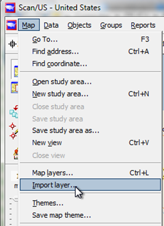
To import locations, choose "Import layer from the Map Menu"
The location data we will choose is the bank branch deposits that we have for all bank locations in the United States as of October 2010, which can be generated from a file of branch bank street addresses and deposit information maintained by the FDIC.
You may decide to choose a different data file, and work the steps with your file as we go through Banks.
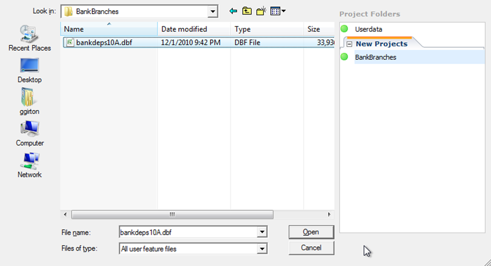
Choose the location file, which must contain latitude/longitude coordinates
Notice the BankBranches project folder in the upper right. Project folders are a Scan/US convenience, so you can keep files for a project in a folder. You can activate (and de-activate) project folders by choosing "Project folders.." from the Tools menu.
However, you don't need to do that here. When you import a map layer file, a new project folder is created, and activated, automatically for you. The green circle means the folder is active.
Choose the file to import, and click "Open". The Import Layer dialog appears (shown below).
Underneath "layer name," replace the filename with a more descriptive name (green arrow below) such as "Bank branch locations (Oct 2010)".
Then you need to set up the roles that the data fields will play. The way to do this is 1: select the field (red circle below left), and 2: click the role button which the field will play (red circle below right). This sets up the role for that field.
The four essential roles are the unique key, the name to be displayed, and the latitude and longitude of the location.
The Import Layer dialog makes an effort to auto-assign these roles to fields with appropriate names. Thus, "Key" is assigned to the field called "key", and (we will find in the next panel when you scroll down) latitude and longitude are already assigned too, since the file has those names for the fields.
However, if we want to see a name for the bank branch, it's necessary to pick a field to play the name role, and you do that below.
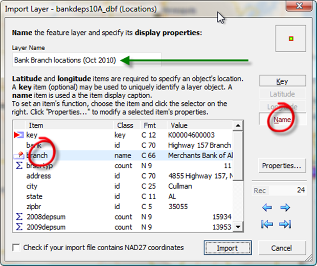
Choose the correct 'role' for each data field
The way the Import Layer works is: first you click the field, e.g. "Key", and then you click the Role each field plays. When you do this for the Key role, it will show the red triangle. When you do it for the name role, you will see a little pushpin appear that indicates what the name field will be, as above.
Finally, scroll down to see that latitude and longitude are already assigned the correct roles.
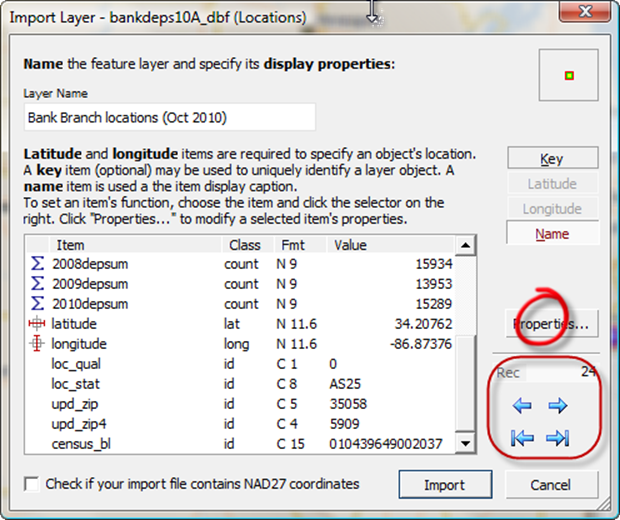
Latitude and Longitude are correctly assigned
Usually they will be pre-assigned, and no action is necessary. However, if in your file the names of latitude and longitude fields are different, you will need to assign them manually by clicking first on the field name for latitude, and then on the latitude button.
Also notice the four blue arrows (within red rectangle, above). The top two blue buttons control stepping through your file record by record, so you can make sure you have the right file. The bottom two toggle between the first and last records in your file.
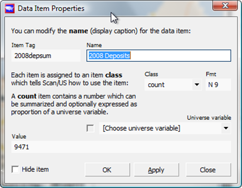
Before you click "Import", you can use the "Properties" button (red circle above) to change the names of some of the fields. In particular, wouldn't it be nice if "2008 depsum" was called "2008 deposit summary"?
Click the "2008 depsum" field, and then the "Properties" button to change the name of it and the other two deposit year variables.
Renaming the layer
This is useful when the field name of the item is cryptic, or if there is more information about the item (such as units) which you wish to add onto the caption.
Also, you may need to change the "type" of some of your fields (assuming you are not importing this bank file, which we license to Scan/US customers in a pre-imported form anyway).
This is true for the field called "brtyp", which we will want to change to "Branch Service Type".
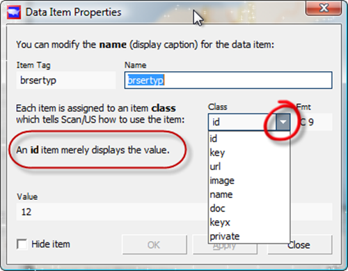
Changing item properties
Click the "Class" dropdown (red circle) and select "id". This is because the branch service type is entered in the file as a number, but it is not the kind of numeric field that you want to calculate a summary, or a statistic for. It is just an ID, so you click ID.
You may notice that as you fly your mouse over some of the other fields in the "Class" dropdown, that descriptions (red rounded rectangle) of some of the other classes appear, such as "URL", or "image". These identify, respectively, URL web links and names of image files that show up in the Quicklook dialog after the file is loaded, that let you click and open a web page, or look at a picture file, when the name of the picture file is specified in your imported database. The banks file does not have these kinds of fields, however.
Now you can click import, and in a second this will load.
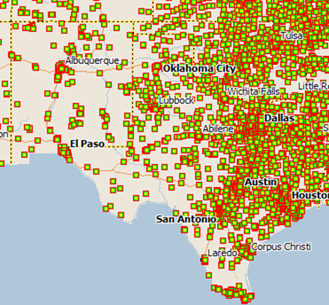
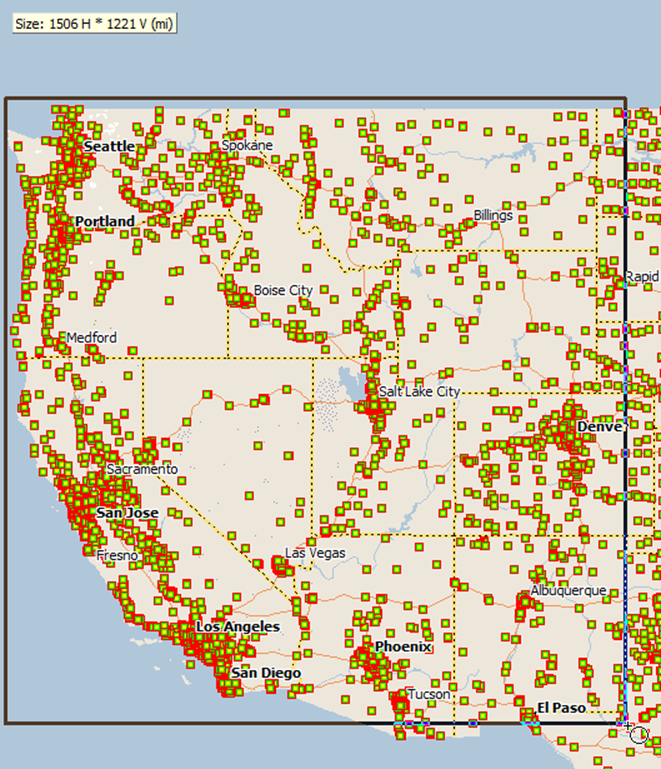
Zoomed in on branch locations in part of Texas
The whole US will be covered with little squares showing bank locations.
Now, so we can show off Scan/US's grouping capability, we'll export data for just some of the bank locations.
Exporting data attached to a location file
We will take data only for the banks which are west of Texas. For the purpose of this example, we will interpret that loosely to mean west of MOST of Texas.
To do this we will create a group of banks, and then operate only on members in that group. Making a group is how Scan/US does multiple selection.
First, we select the "group by rectangle" grouping submode.
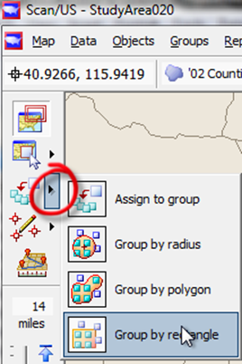
Select 'group by rectangle' in group mode
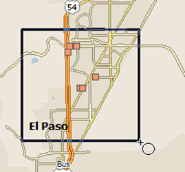
Then, clicking at the upper left of the rectangle to draw it, draw a rectangle (from up near Seattle) down to El Paso to get those banks west of Texas.
Making a big group of banks west of Texas
The "New Group" dialog appears.
In place of the group name "Group001" enter the name "West of Texas." You can give the grouping a name, too: Bank Example.
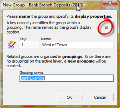
Naming the new group
Click OK. The banks in the new group will be shown with little salmon colored squares like the one circled in red (above). By the way, if you want to change the group indicator for locations to be a different color, or a different shape, that red-circled area (above) is a button. You can press it, and change the type of group marker for the location.
Since we missed a few locations down here in southern New Mexico, we'll just draw another small rectangle to bring those in.
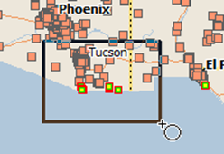
Adding some more banks to the group
They're added to the group called West of Texas
.
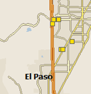
Just to make sure you've got this right, select framing mode and draw a rectangle to zoom in to El Paso
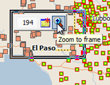
**
We can make sure we don't have any banks that are actually In Texas, and that none of the other banks have escaped our grasp.
Just to get a little more detail, we can make a small study area. From the Map Menu, choose New Study Area. A new study area opens, but the group of banks is not shown.
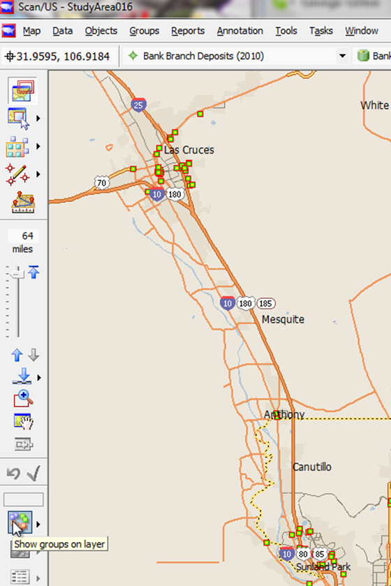
Zooming in to get a closer look
To see the group in the new study area, we have to click "Show groups on layer" over on the left to activate that set of groups, which is called a "grouping".
Activating the grouping in a new study area
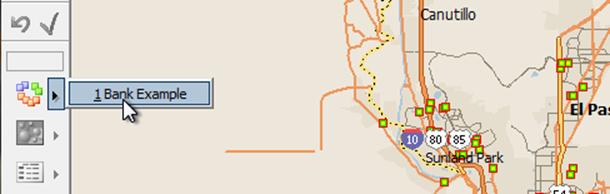
A "grouping" is a setof groups. So, click the black triangle to see the groupings on the layer, and activate the grouping you named earlier as "Bank Example".
You can see from the map that it looks like we did by accident include some banks in Texas.
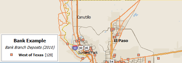
Banks within Texas are not west of Texas!
We'll make a new group to clean those up.
Choose "New Group" from the Groups Menu, and change the name from Group002 to Texas Banks. Then click OK.
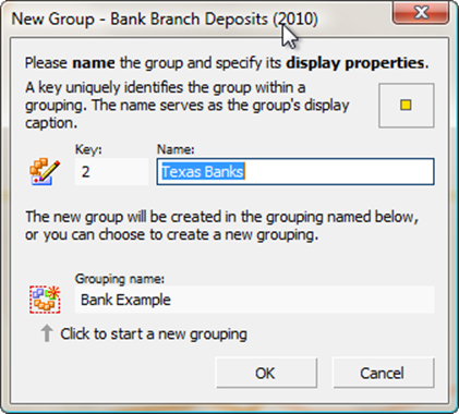
Creating a new group
Next, use the same group-by-rectangle tool (which should still be active) to draw around the Texas banks.
Adding to the new group
It will add them to the group called "Texas Banks"
El Paso banks are in Texas
And this way we won't have any Texas Banks in our "West of Texas" group.
Now we have created a grouping of banks, called "Bank Example," and a group within that grouping called "West of Texas".
Step 2: Export data attached to each location
Export Bank Branch Deposit data for 16,228 banks west of Texas (not including any banks within Texas).
Point Data Export
From the Data Menu, Choose Export Data. The Export Data dialog appears.
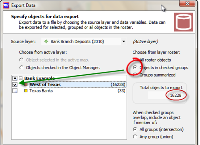
Export data, objects in checked groups
In the column on the right, "Choose from layer roster", click the "Objects in checked groups" (red circle) to see the "Bank Example" grouping, and put a check next to the group called "West of Texas" (green arrow). Notice that you have a large number of total objects to export (red oval). This is the number of banks west of Texas. Remember that the number for "Texas Banks" is just the few banks around the edge that you put into a group. It isn't anywhere near all the banks in Texas. But you aren't going to pick that group anyway.
Click "Next" to go to the "Specify data variables" page:
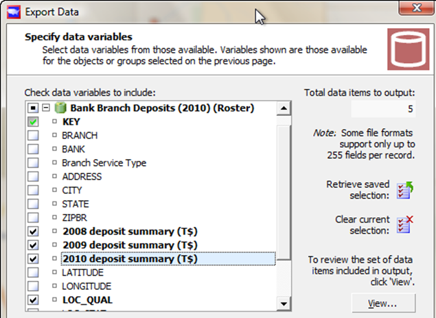
Specify data variables: KEY and deposit summaries
Notice that there is a green checkmark next to the KEY field. The key will always be exported: you never need to choose it specifically, and you will not be able to omit it.
The main data variables we are looking for are the deposit summaries. Click the checkbox next to each one to include it in the export. Also, we will export location quality so in the future we at least have a chance to double check how accurately any particular bank location is depicted. The Loc_Qual field was put there by a geocoder, and something to keep in the back of your mind, is that the accuracy of a geocoder's result is known, and kept track of (and is not perfect).
The two buttons on the right, next to "Retrieve saved selection" and "Clear current selection" can be useful when there are many data items to select. The "Clear" button makes sure you are starting from a blank slate of variables, and the "Retrieve" button can save a selection you have used before (and saved at the next step, where you also specify the filename). We are not going to use these two buttons in our example.
Click "Next" to get to the screen where you will name and save the exported file.
Change the export filename from D-export.csv to "BanksWestOfTexas.csv"
and click "Export" to export to that data file.
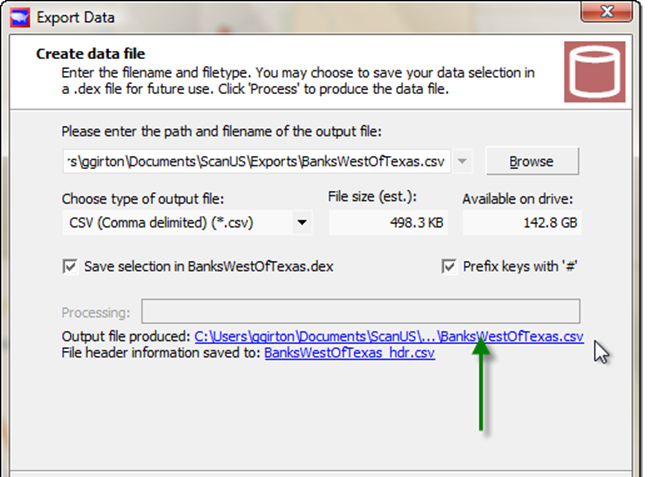
Create data file
When it is done, two blue "link buttons" will appear.
To see the exported values, click the blue link button (green arrow above) : this will open the database in Excel.
The spreadsheet shows the branches and all of their deposits.
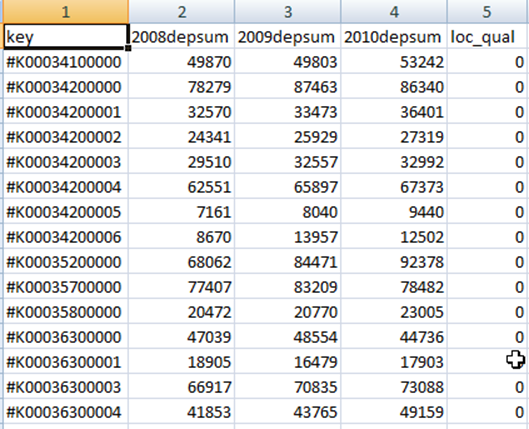
Branches and their deposits
We'll go back to Scan/US, close that Export Data Dialog, and move on to the next step, which is exporting demographic data for the trade areas near the banks.
Step 3: Create a ring around each location
This step is facilitated by another thing you can do with Scan/US, which is to copy those objects, the bank branch locations, to create a new layer of rings.
Create a three-quarter-mile ring around each bank location.
From near the bottom of the Scan/US Objects menu, choose Copy Objects. The Copy Objects dialog appears:
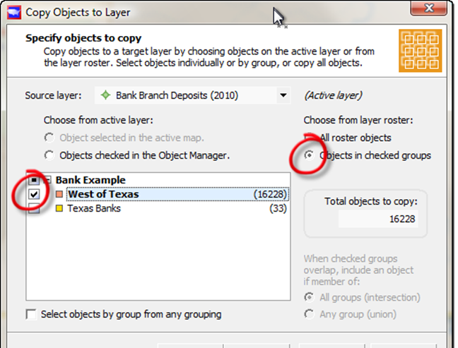
Copy Objects: Specify object to copy
In the right column, underneath "Choose from layer roster", select "Objects in checked groups."
Then you will see the Bank Example grouping on the left. Click the "+" sign next to it to expand it into its component groups.
Then you will be able to select the group "West of Texas" (other red circle), and click Next.
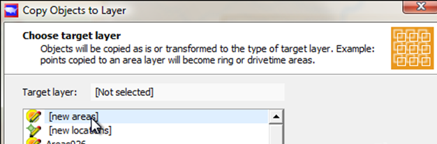
Target layer: New Areas
The target layer you will choose is "New Areas". New Areas lets you create new ring areas, OR new Drivetimes. You will chose the Ringareas tab.
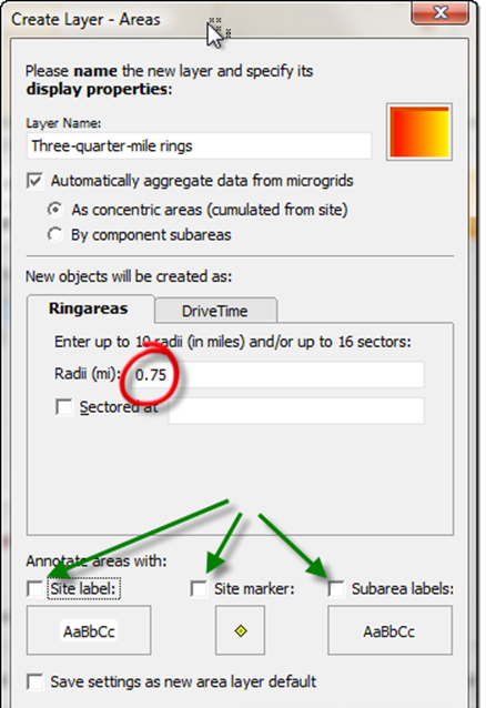
Make a three-quarter-mile ring (red circle), with no labels (green arrows)
Next to "Radii", enter the value 0.75 (red circle), for three-quarters of a mile. Also, clear the checkboxes next to site label, site marker, and subarea labels. You don't need any of these to export the data, and there is already a point marking the center, and with only one subarea (.75 miles), you don't need to label it separately.
Click OK to get back to the Copy Objects dialog.
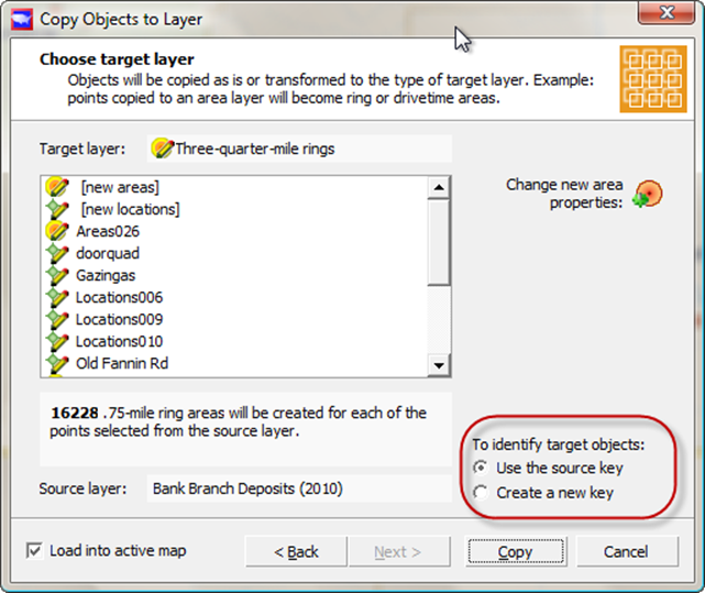
Use the source key
Now your new layer is set up, and you can click Copy. Notice in the lower right-hand corner you have an option to re-key all the objects in the new layer. If you do that here, you will lose any reference back to which bank corresponds to each circle. You should leave "Use the source key" selected. Also, there is a button above that, "change new area properties", which we will not be using in this example.
Click copy to create the new layer. Since there are a lot of objects, it will take a few moments to build the cross reference. What Scan/US does when creating a new geographic layer is to aggregate ALL the demographic data from ALL the underlying databases into the new geographic layer objects, in this case three-quarter-mile rings surrounding banks that are west of Texas. In order to do that, it needs to build a cross-reference to the underlying MicroGrid containers.
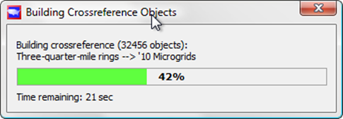
Building cross-reference -- surprisingly fast for so many ring objects.
What Scan/US is doing right now is creating new rings and summarizing the demographic data from the underlying microgrid level to those rings. At just three-quarters of a mile radius, you may not be able to see them. To see them, you may need to zoom in. (Actually, we will create a new study area to get more detail)
Make sure you are in framing mode:
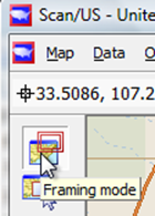
Framing mode to zoom
Then draw a rectangle around Las Cruces (or other city in your map) and choose New Study Area.
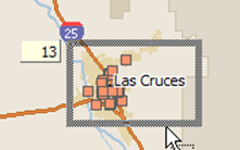
With the rectangle drawn, choose New Study area from the Scan/US Map menu
Then you will be able to see the ring around each point.
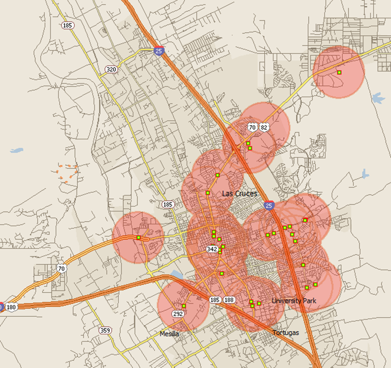
Ring areas around each bank
Let's look at data for one of the rings.
Make sure you are in Select object mode,
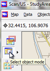
Go into select mode to select a single object
and click on a ring to bring up the selection tree, then choose the bank:
Here we choose Bank of the Rio Grande (in the upper right-hand corner of the map).
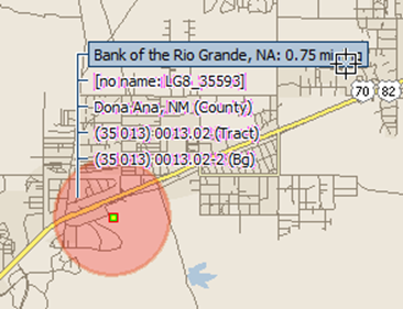
The selection tree shows what's on the ground at that location
On the data menu, choose Quicklook, and you can see the 2010 Demographics
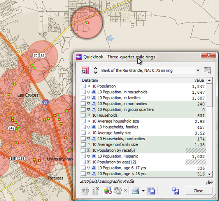
Look at the demographics in the vicinity of any branch
By looking at any of the demographic values, we can see for example the 2010 pop 1,847 in 631 households for that ring.
Of course you don't have to look at an object's data in Quicklook to export the data, this is just a quick detour so you can see the data is there.
Step 4: Demographic Data Export,
From the Data Menu choose Export data,
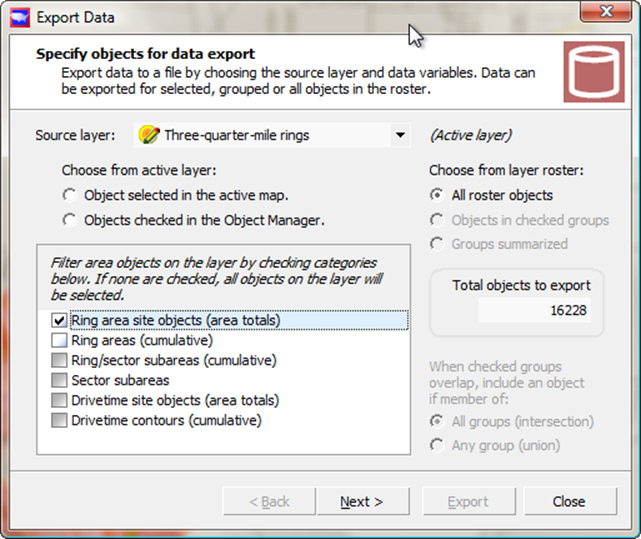
Just choose the ring area site object to get the data
Here, you choose 'All roster objects', rather than the grouped objects because it's a new layer -- of rings -- that we created from the West-of-Texas group to begin with.
When you do this, you will notice a list of checkbox options to filter the area objects. These options are present to deal with the fact that area objects - both rings and drivetimes - have subareas that can be selected separately. Here, just choose the area totals for export.
You can see the by-now-familiar number 16228 pop up (for you it may be a different number), and then click "Next" to choose data items for export.
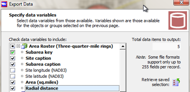
From the area roster, you can choose facts about the area
We automatically get the Key, which is called the "Subarea key", and in addition we will check off the site and subarea caption, and the area in square miles (which in this case is always going to be the same, but for concentric rings would not be), and the radial distance so we'll know it's a .75 mile radius
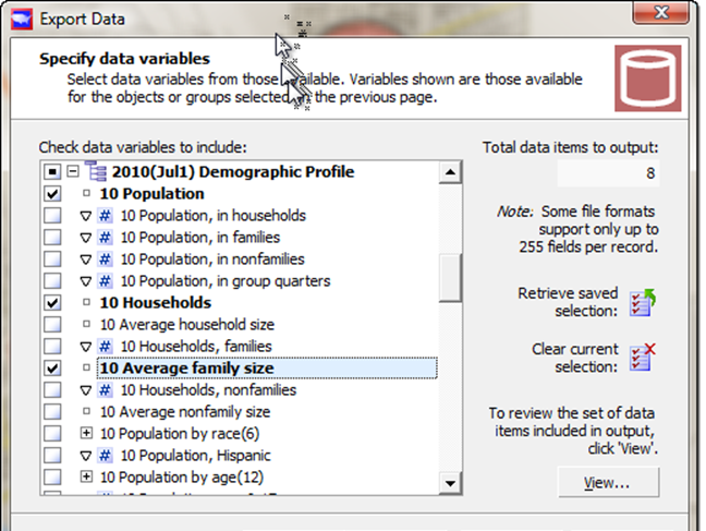
Scroll down to get demographic data items from other datalists
Then we'll scroll down and expand the 2010 (Jul1) Demographic Profile (click the plus next to it), and check off the population and the households and average family size, and you can scroll down and get the median income.
Click NEXT to get the "Create data file" page
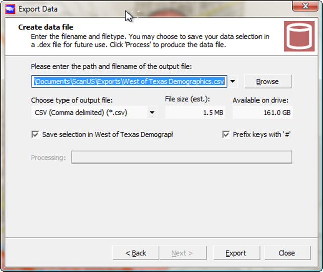
Choose a good filename for export
Enter the filename "West Of Texas demographics.csv", click Export, and that is going to be about a 1.5 megabyte sized file because it has all that data in it, it's 8 data items for just over 16,000 objects (three-quarter-mile rings).
The export will not be instantaneous.
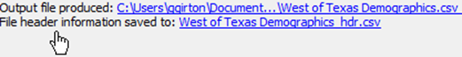
And when this is done it'll have another little blue link button under that processing bar and we'll be able to click on that and bring it up in Excel.
Now you may notice there are TWO link buttons. The top one is the data file, and the bottom one the "header" for the data file, which describes the fields more fully.
Most people are more interested in the TOP file -- but we'll look at the bottom one first:
Click on the bottom file to look at the header information -- this is the database schema
So when you look at the header file, it will look like this:
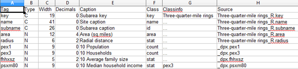
The header file describes the variables
This shows the "Tag", which is the name used in the first row of the data file, and other information about the data item, including whether the field is character 'C' or numeric 'N', the number of decimal places, the human-friendly name or "Caption", the class of data item it is, and its data item source - so you can see what data list it comes from, or whether it comes from a roster of geographic objects (i.e. has a big "_R" in the source name).
Then, below, you can see the three-quarter-mile demographics for the banks west of Texas (in October of 2010), the population, number of households, average family isze, and median household income.
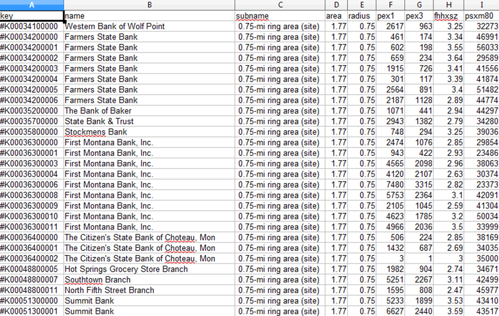
The top link brings up the data file itself
And since you have the bank #K-number keys, you can, if you wish, do a copy-and-paste within the two Excel data files, to combine this data file with the one you exported earlier with bank deposit information, and know practically everything about Banks West of Texas.